- Classification 모델
- class에 따라 data instance를 잘 분류하는 것. feature space에서 분류하는 boundary 혹은 hyperplane을 찾는 것.
- 모델 종류: linear model, non-linear model, tree model
- 에러 계산 방식(최적화 방식)
- error-rate, 거리 계산
- probability (data point를 가지고 확률 분포 결정)
- 영역을 divide-and-conquer 전략으로
- gradient discent 방식으로
1. Zero-R(0R)
label의 각 class 개수만 따져서 그 확률로 판단. minimum(baseline) 성능
ex. class{ yes, no }에서 yes가 9개, no가 5개인 경우: 9/14=약 65% 확률로 yes로 판단
2. One-R(1R)
제일 좋은 feature 하나만 고름. 선택 기준은 error rate / entropy
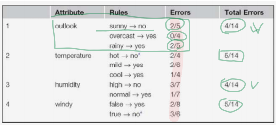
각 feature(ex. outlook)의 속성값 각각(ex. sunny, overcase, rainy)에 대하여
더 많은 쪽의 class(yes or no)로 rule을 만들었을 때의 각각의 errors(확률) 더하여 total errors를 구함
각 feature의 total errors를 비교하여 가장 error가 작은 feature를 선택(ex. outlook)
- numeric attribute가 있는 경우?
- Discretization을 한다: categorical / discrete data로 변환
- class가 바뀔 때마다 하나의 카테고리로
- overfitting 문제: feature의 value 값이 많을 수록 overfit 가능성이 높다. (=highly branching attributes do not usually perform well on test samples)
- 최악의 욕심쟁이 feature: 주민번호(ID) -> overfit, 새로운 데이터 적용이 불가능하므로 사용하면 안됨.
- minimum limit을 설정하고 class가 그만큼 나타난 지점을 기준으로 나눔. 이때 바로 다음도 같은 class이면 포함시킴
- ex) yes no yes yes yes | no no yes yes yes | no yes yes no (partition limit = 3)
- yes | yes | no
- yes |(=이때의 temperature라는 feature의 값이 77.5) no가 되고
- rule은 77.5이하는 yes, 초과는 no가 된다.
- class가 바뀔 때마다 하나의 카테고리로
- Discretization을 한다: categorical / discrete data로 변환
3. Decision Tree
Divide-and-conquer(분할정복) 방법: 한 번에 하나씩 best feature를 선택. 이것을 recursive하게 반복. 결국 top-n개의 best feature들의 복합체.
feature space를 직사각형 모양으로 영역을 나누어 감.
- Pruning: postpruning (backward pruning) / prepruning (forward pruning) -> overfitting 방지
- feature 선택 기준: Entropy(information gain) 또는 Gini
- Entropy
- |정보가 없을 때 혼란도 - 정보가 있을 때 혼란도| = 정보의 가치 (bit)
- 1 bit: 아무런 정보가 없을 때의 '불확실성의 크기'
- 특정 사건의 entropy 값: -log₂P (사건이 발생할 확률이 P)
- attribute(feature)의 entropy H = -∑P log₂P
- information gain(R): H_before - H_after
- H는 작을수록 R은 클수록 class를 잘 분별하는 feature
- gain ratio: value의 개수가 많을 수록 entropy 값을 상쇄하기 위해서 gain을 나누는 값 (overfitting 방지)
- Gini (Simpson's diversity index, one minus the repeat rate)
- diversity index: 두 번째로 선택한 것이 첫 번째와 다른 class일 확률
- Gini = 1 - (그 안에서 같은 게 두 번 나올 확률들의 합) = 1 - ∑P^2 : 최대 0.5
- 각 split의 diversity를 Gini(before split) - Weighted Average of (Gini(left child) + Gini(right child))로 평가해서 최소 다양성 추구.
- gini 사용 예시 - CART(Classification and Regression Tree): 단일 input에 대한 함수로 노드를 나누는 이진트리. n개의 case와 r개의 variable에 대하여 nr개의 possible split에 대하여 모두 평가.
- Entropy

- impurity(purity)의 세 가지 판단 기준: Misclassification, Gini, Information gain

4. Probabilistic modeling
- Naive Bayesian classifier(NBC)
error rate에 의해서 P를 계산P(H | e)를 구하고 그 확률에 따라 classification을 함H: hypothesis(-> class), E: evidence일 때 P(H|E) = P(E|H) P(H) / P(E)
- P(H|E): posterior probability
- P(E|H): conditional probability
- P(H): prior probability
- P(E|H) P(H): likelihood of H


- 데이터가 numerical한 경우: 확률 분포함수(PDF)를 사용
5. Rule(classification rule)
가장 일반적인 "if-then rule": if A, then B
A: condition part, antecedent, premise, left-hand side(LHS)
B: consequent, conclusion, action, righ-hand side(RHS)
Rule set: {R1, R2, ..., Rn} // 각 rule 내에서는 conjunctive(∧), 각 rule들은 서로 disconjunctive(∨)
- feature space가 2차원(p1, p2)일 때
- 1) if p1=C and p2=T, then Class1 → most specific, covers just 1 case
- 2) if *(whatever, default rule), then Class1 → most general, covers all the cases
- rule의 목표: cover하는 것이 maximally general and accurate
- accuracy와 coverage의 trade off! 어디서 멈출 것인지 알고리즘으로 판단..
- feature space에서 retangular한 영역을 만든다 -> DT와의 차이점: DT는 전체를 다 cover
- Rule을 만드는 알고리즘
- PRISM: 아무 것도 없는 상태에서 R이 perfect(accurate)해질 때까지 rule을 하나씩 추가
- PART: DT를 만들고 largest leaf를 가지고 rule 추가
- Grow and Prune: Grow 단계에서 PRISM을 사용해서 class C에 대한 best perfect rule 생성 후 Prune 단계에서 rule R의 worth인 w(R)을 계산. R이 없을 때의 w이 더 크면 R 제거를 반복. 마찬가지로 다른 class에 대하여 반복.
- JRip(Ripper): 중요한 것에 대해서만 rule 결정. 마지막 rule은 default rule (간단하고 정확도가 높음)
- J48: DT
Association rule
f1과 f7이 연관성이 있는 경우: if f1, then f7
ex) Market Basket Analysis(장바구니 분석), Recommender system
발생빈도를 가지고 attribute들 간의 연관성을 추정
frequency의 기준: Minimum suppoer (같이 발생한 최소 횟수)
이를 바탕으로 frequent item set을 추출한 후 associative rules로 표현
A-Priori Algorithm: frequent item set을 찾는 알고리즘
- issues:
- complexity 문제: n개의 attribures에 대하여 O(n^2)
- 줄이는 방법: A-Priori Algorithm
- A Prori Property: 어떤 itemset이 frequent하다면 그 itemset의 모든 부분집합(공집합 제외)은 also frequent 하다.
- A Priori Algorith: frequent하지 않은 부분집합을 제거
- interestingness 문제
- 인기 항목 간에 아무런 연관이 없이 함께 발생 가능
- 확률에서의 correlation(=기계학습에서의 Lift) 이용: P(a1, a2) / P(a1) P(a2) > 1이면 연관 positive, = 1이면 서로 독립적, < 1이면 negative
- 또는 conviction(확신도) 사용
- complexity 문제: n개의 attribures에 대하여 O(n^2)
6. Linear model
Linear Regression(선형 회귀): 수치 예측에 쓰임 (not classifier)
- y = w1*x + w0
- error(예측값과 실제값의 차이)의 합을 최소화하는 w0, w1 값을 구함
- feature의 개수가 n이 커질 수록 모델이 복잡해짐 -> feature selection
- w(coefficient)를 어떻게 구할 것인가?
- maximum likelihood 방식: 확률 이용 -> Logisitc Regression
- gradient descent 경사하강법: squared error를 cost function으로 해서 -> Perceptron의 delta rule, MLP의 back propagation 등
6-1. Logistic Regression (classifier)
Linear regression으로 classification하는 법: class를 numerical data 0, 1로 바꾸고 regression을 수행하여 예측값 생성
단점: 0~1 범위를 벗어날 때 판단하기 어려움. error값을 확률적으로 계산하기 힘듦, 0을 사용하기 어려움(odd ratio = p/(1-p))
-> 따라서 통계적 기술인 Logistic regression을 사용
- logit transformation(odd ratio에 log를 씌움): ln(p/(1-p)) = ax+c //p = a1x1 + a2x2 + ... + anxn + c
- p/(1-p) = e^(ax+c)
- p(y=1|x) = 1 / (1+e^(-(ax+c))): sigmoid 함수
- sigmoid 함수 그래프: input이 ax+x, output이 y=1일 확률
- feature space는 확률적인 분포로 이루어져 있고, 어디를 찍더라도 확률값이 나옴
- p=0.5인 line : decision boundary
- [-∞, ∞] -> [0, 1]로: 스퀴즈함수라고도 부름
6-2. Perceptron
인간의 뇌: 뉴런들은 시냅스로 연결되어 있음.
시냅스 연결이 기억과 정보처리의 핵심이며, 시냅스가 연결되는 것이 바로 학습
- Perceptron에서 모델링하는 것:
- 뉴런
- 시냅스의 연결강도: weight
- learning rule: 경험에 의해 어떻게 연결강도가 강화/약화되는지
- y = f(∑xiwi - θ ) = 0 or 1
- f: activation function(활성 함수): 주로 sigmoid / hard-limit(=step) function
- θ: threshold
- y = w1a1+w2a2+w0 = 0 에서 y = w1a1+w2a2 = -w0 = -θ 로 변형
- ∑wa를 θ 기준으로 y=0 or 1 (x좌표 w0(=θ)를 기준으로 하는 hard-limit 함수)
- w를 구하는 방법: Delta Rule
- 연결 가중치의 값을 적응적으로 update
- input과 expected output의 오차를 줄여나가는 방향으로 값 조정
- 처음에는 임의의 w값
- wi = wi + ⧍i(= learning rate * 에러값(기댓값-실제값) * xi)

logistic regression과의 차이점: feature space는 확률적 공간이 아니며 두 개의 class만 구분하는 decision boundary를 찾고자 함.
perceptron의 강력한 장점은 Network: NN으로 진행
한계: XOR 해결 불가능 -> 여러 perceptron을 조합시킴으로써 non-linear 형태를 만들어냄 (MLP)
'대학공부 > 기계학습' 카테고리의 다른 글
| Deep NN (0) | 2023.10.11 |
|---|---|
| Feature selection, SVM, 앙상블 (0) | 2023.10.11 |
| Evaluation (0) | 2023.10.11 |
| Classification(2) (0) | 2023.10.10 |
| 기계학습(ML)이란? (0) | 2023.10.10 |

