실습 4차시: 퍼셉트론, MLP

퍼셉트론이란?

퍼셉트론은 신경망의 가장 기초가 되는 기본 단위입니다. 생물학적 뉴런의 작업을 시뮬레이션하는 인공 뉴런이라고 할 수 있습니다.

퍼셉트론은 3가지 구성요소로 이루어져 있습니다.

• 입력(Inputs)
• 가중치(Weights)
• 출력(Output)

---

Perceptron Class

Perceptron 클래스 작성하기

lines = []

class Perceptron:

  def __init__(self, num_inputs = 3, weights = [1,1,1]):

    self.num_inputs = num_inputs

    self.weights = weights

  def weighted_sum(self, inputs):

    weighted_sum = 0

    for i in range(self.num_inputs):

      weighted_sum += inputs[i] * self.weights[i]

    return weighted_sum

  def activation(self, weighted_sum):

    if weighted_sum >= 0:

      return 1

    else:

      return -1

  def training(self, training_set):

    foundLine = False

    while not foundLine:

      total_error = 0

      for inputs in training_set:

        prediction = self.activation(self.weighted_sum(inputs))

        actual = training_set[inputs]

        error = actual - prediction

        total_error += abs(error)

        for i in range(self.num_inputs):

          self.weights[i] += error * inputs[i]

      slope = -self.weights[0] / self.weights[1]

      intercept = -self.weights[2] / self.weights[1]

      y1 = (slope * 0) + intercept

      y2 = (slope * 50) + intercept

      lines.append([[0, 50], [y1, y2]])

      if total_error == 0:

        foundLine = True

위 클래스의 구현 과정:

가중합(Weighted Sum) 구하기

입력과 가중치를 출력으로 변환하기 위해서는, 우선 각 입력에 대한 가중치를 더해서 가중합을 계산해야합니다.

weighted sum = x_1 * w_1 + x_2 * w_2 + ... + x_n * w_n

위 수식을 구현해봅니다.

 

활성화 함수(Activation Function)

퍼셉트론의 출력은 앞에서 계산한 가중합으로부터 결과값을 생성함으로써 결정되게 됩니다. 결과값을 생성해주는 함수를 활성화 함수라고 합니다.

다양한 활성화 함수들이 존재하는데, 이번 실습에서는 Step Activation Function을 사용합니다.

• 입력에 대한 퍼셉트론의 가중합이 양수라면 1을 반환합니다.
• 입력에 대한 퍼셉트론의 가중합이 음수라면 -1을 반환합니다.

활성화 함수를 perceptron class에 구현해봅니다.

 

오차(Error) 구하기

퍼셉트론의 출력값과 학습 데이터의 타겟값이 일치하지 않을 때, 오차를 구할 수 있습니다. 오차는 해당 모델과 실제 데이터간의 차이를 나타냅니다.

우리의 목표는 퍼셉트론을 오차가 작아지는 방향으로 학습시키는 것입니다. 훈련 오차는 실제 레이블 값에서 예측된 레이블 값을 빼서 계산됩니다.

training error = actual label - predicted label

Step activation function을 사용하는 퍼셉트론이 만드는 오차는 다음의 네 가지 경우를 띕니다.

 

가중치 수정하기

퍼셉트론 학습의 목표는 가중치를 올바른 방향으로 수정해서, 정답을 출력하는 최적의 가중치를 찾는 것입니다.

최적의 가중치를 찾는 방법 중, 가장 널리 사용되고 있는 것이 바로 경사하강법(Gradient Descent)입니다. 이번에 우리는 Step Activation Function을 사용하기 때문에, 경사하강법 중 Delta Rule을 통해 가중치를 학습시킬 것입니다.

Delta rule은 다음의 간단한 규칙을 통해 가중치를 수정하게 됩니다.

weight = weight + learning rate * (error * input)

퍼셉트론은 모든 결과값을 정확하게 예측할 때까지 가중치를 계속 조정합니다. 그렇기 때문에 학습이 완료되기 전에 데이터셋을 여러번 반복하여 학습시켜야 할 수도 있습니다. 위 perceptron class에 학습시키는 코드를 수정해봅니다.

 

편향치(Bias)

그러나 퍼셉트론의 정확도를 높이기 위해 약간의 조정이 필요한 경우가 있습니다. 이를 위해 우리는 퍼셉트론에 편향치를 추가합니다.

편향이 추가된 가중합의 식은 다음과 같습니다.

weighted sum = x_1 * w_1 + x_2 * w_2 + ... + x_n * w_n​ + w_b

다음 두 가지 변경사항만 고려하면 앞서 구현한 퍼셉트론에 편향을 적용할 수 있을 것입니다.

• 입력 데이터의 마지막에 1을 추가합니다 (이제 2 대신 3 개의 입력이 있음).
• 가중치 목록에 편향 가중치를 추가합니다 (이제 2 개 대신 3 개의 가중치가 있음).

위 perceptron class에 해당 코드를 추가해봅니다.

 

퍼셉트론을 통한 선형 분류

퍼셉트론의 훈련 과정을 더 잘 이해하기 위해 퍼셉트론의 훈련 과정을 시각화 해봅니다.

가중치는 훈련 과정 전반에 걸쳐 변경되므로 해당 가중치를 의미있게 시각화 할 수만 있다면 기울기-절편 형식을 사용하여 선을 나타낼 수 있다는 것을 알고있을 것입니다. 퍼셉트론의 가중치는 퍼셉트론이 나타내는 선의 기울기와 절편을 찾는 데 사용할 수 있습니다.

• 기울기 = -self.weights[0] /self.weights[1]
• 절편 = -self.weights[2] /self.weights[1]

위 perceptron class에 해당 코드를 추가해봅니다.

---

퍼셉트론 학습시키기

실제 대부분의 기계학습에서 사용하는 데이터는 tabular 형태를 띄고 있지만, 이번 실습에서는 입력값과 출력값을 dictionary 형태로 표현한 데이터셋을 사용하도록 하겠습니다. 우리가 사용할 데이터셋은 다음과 같은 형태를 지닙니다.

training_set = {(18, 49): -1, (2, 17): 1, (24, 35): -1, (14, 26): 1, (17, 34): -1}

import random

def generate_training_set(num_points):

  x_coordinates = [random.randint(0, 50) for i in range(num_points)]

  y_coordinates = [random.randint(0, 50) for i in range(num_points)]

  training_set = dict()

  for x, y in zip(x_coordinates, y_coordinates):

    if x <= 45-y:

      training_set[(x,y,1)] = 1

    elif x > 45-y:

      training_set[(x,y,1)] = -1

  return training_set

#training 데이터셋을 generate_training_set 함수를 사용하여 30개의 데이터를 생성합니다.

training_set = generate_training_set(30)

import seaborn

import matplotlib.pyplot as plt

x_plus = []

y_plus = []

x_minus = []

y_minus = []

for data in training_set:

  if training_set[data] == 1:

    x_plus.append(data[0])

    y_plus.append(data[1])

  elif training_set[data] == -1:

    x_minus.append(data[0])

    y_minus.append(data[1])

   

fig = plt.figure()

ax = plt.axes(xlim=(-25, 75), ylim=(-25, 75))

plt.scatter(x_plus, y_plus, marker = '+', c = 'green', s = 128, linewidth = 2)

plt.scatter(x_minus, y_minus, marker = '_', c = 'red', s = 128, linewidth = 2)

plt.title("Training Set")

plt.show()

# 퍼셉트론을 만들고 데이터에 훈련시켜 봅니다.

perceptron = Perceptron()

perceptron.training(training_set)

아래 코드는 구현한 퍼셉트론이 가중치를 변화시켜가며 최적의 선을 그리는것을 시각화 한 것입니다.

import seaborn

import matplotlib.pyplot as plt

import matplotlib.animation as animation

from matplotlib import rc

from IPython.display import HTML

import random

x_plus = []

y_plus = []

x_minus = []

y_minus = []

for data in training_set:

  if training_set[data] == 1:

    x_plus.append(data[0])

    y_plus.append(data[1])

  elif training_set[data] == -1:

    x_minus.append(data[0])

    y_minus.append(data[1])

fig = plt.figure()

ax = plt.axes(xlim=(-25, 75), ylim=(-25, 75))

line, = ax.plot([], [], lw=2)

fig.patch.set_facecolor('#ffc107')

plt.scatter(x_plus, y_plus, marker = '+', c = 'green', s = 128, linewidth = 2)

plt.scatter(x_minus, y_minus, marker = '_', c = 'red', s = 128, linewidth = 2)

plt.title('Iteration: 0')

plt.close()

def animate(i):

    print(i)

    line.set_xdata(lines[i][0])  # update the data

    line.set_ydata(lines[i][1])  # update the data

    return line,

def init():

    line.set_data([], [])

    return line,

ani = animation.FuncAnimation(fig, animate, frames=len(lines), init_func=init, interval=100, blit=True, repeat=False)

rc('animation', html='jshtml')

ani

---

과제

이번 과제에서는 AND, OR, XOR 데이터에 대해 Perceptron으로 분류해보도록 하겠습니다. 아래 함수들은 과제에서 시각화를 도와주는 함수들입니다.

def plot_data(x, y):

  plt.scatter([point[0] for point in x], [point[1] for point in x], c=y, cmap=ListedColormap(['#FF0000', '#0000FF']))

  plt.show()

from matplotlib.colors import ListedColormap

# Perceptron의 decision boundary를 그려주는 함수입니다.

# 함수 출처: http://scikit-learn.org/stable/auto_examples/classification/plot_classifier_comparison.html

def plot_decision_boundary(classifier, X, y, title):

  xmin, xmax = np.min(X[:, 0]) - 0.05, np.max(X[:, 0]) + 0.05

  ymin, ymax = np.min(X[:, 1]) - 0.05, np.max(X[:, 1]) + 0.05

  step = 0.01

  cm = plt.cm.coolwarm_r

  thr = 0.0

  xx, yy = np.meshgrid(np.arange(xmin - thr, xmax + thr, step), np.arange(ymin - thr, ymax + thr, step))

  if hasattr(classifier, 'decision_function'):

    Z = classifier.decision_function(np.hstack((xx.ravel()[:, np.newaxis], yy.ravel()[:, np.newaxis])))

  else:

    Z = classifier.predict_proba(np.hstack((xx.ravel()[:, np.newaxis], yy.ravel()[:, np.newaxis])))[:, 1]

  Z = Z.reshape(xx.shape)

  plt.contourf(xx, yy, Z, cmap=cm, alpha=0.8)

  plt.colorbar()

  plt.scatter(X[:, 0], X[:, 1], c=y, cmap=ListedColormap(['#FF0000', '#0000FF']), alpha=0.6)

  plt.xlim(xmin, xmax)

  plt.ylim(ymin, ymax)

  plt.xticks((0.0, 1.0))

  plt.yticks((0.0, 1.0))

  plt.title(title)

 

1. AND 데이터로 퍼셉트론 학습

1. 데이터를 생성합니다. (and_data, and_labels)
2. plot_data 함수를 사용하여 데이터 시각화해봅니다.
3. scikit-learn의 Perceptron 모델을 생성하고 (모델의 이름은 perceptron_and) 데이터에 .fit()해봅니다. 다큐멘테이션
4. .score()로 데이터에 대해 정확도를 출력합니다.
5. plot_decision_boundary() 함수를 사용하여 훈련된 perceptron의 decision boundary를 시각화하고, 시각화된 plot을 바탕으로 올바르게 분류가 되었는지 서술합니다.

import numpy as np

and_data = np.array([[0, 0], [1, 0], [0, 1], [1, 1]])

and_labels = np.array([0, 0, 0, 1])

plot_data(and_data, and_labels)

from sklearn.linear_model import Perceptron

perceptron_and = Perceptron()

perceptron_and.fit(and_data, and_labels)

perceptron_and.score(and_data, and_labels)

1.0

plot_decision_boundary(perceptron_and, and_data, and_labels, 'AND')

 

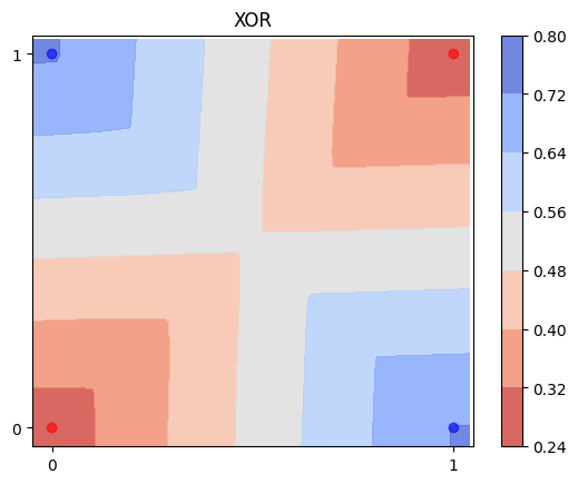
2. XOR 데이터로 퍼셉트론 학습

1. 데이터를 생성합니다. (xor_data, xor_labels)
2. plot_data 함수를 사용하여 데이터 시각화해봅니다.
3. scikit-learn의 Perceptron 모델을 생성하고 (모델의 이름은 perceptron_xor) 데이터에 .fit()해봅니다. 다큐멘테이션
4. .score()로 데이터에 대해 정확도를 출력합니다.
5. plot_decision_boundary() 함수를 사용하여 훈련된 perceptron의 decision boundary를 시각화하고 시각화된 plot을 바탕으로 올바르게 분류가 되었는지 서술합니다.

xor_data = np.array([[0, 0], [1, 0], [0, 1], [1, 1]])

xor_labels = np.array([0, 1, 1, 0])

plot_data(xor_data, xor_labels)

perceptron_xor = Perceptron()

perceptron_xor.fit(xor_data, xor_labels)

perceptron_xor.score(xor_data, xor_labels)

0.5

plot_decision_boundary(perceptron_xor, xor_data, xor_labels, 'XOR')

 

hidden_layer_sizes 파라미터를 조정하지 않은 MLP 모델을  XOR 데이터에 .fit()

from sklearn.neural_network import MLPClassifier

MLPclassifier_xor = MLPClassifier(random_state=42).fit(xor_data, xor_labels)

MLPclassifier_xor.score(xor_data, xor_labels)

1.0

plot_decision_boundary(MLPclassifier_xor, xor_data, xor_labels, 'XOR')

hidden_layer_sizes 파라미터를 다양하게 조정한 MLP 모델을  XOR 데이터에 .fit()

1. 많게 설정

MLPclassifier_xor_1 = MLPClassifier(random_state=42, hidden_layer_sizes=(200,200,200)).fit(xor_data, xor_labels)

MLPclassifier_xor_1.score(xor_data, xor_labels)

1.0

plot_decision_boundary(MLPclassifier_xor_1, xor_data, xor_labels, 'XOR')

2. 적게 설정

MLPclassifier_xor_2 = MLPClassifier(random_state=42, hidden_layer_sizes=(5,)).fit(xor_data, xor_labels)

MLPclassifier_xor_2.score(xor_data, xor_labels)

0.5

plot_decision_boundary(MLPclassifier_xor_2, xor_data, xor_labels, 'XOR')